Introduction
Sometimes, when I’m reading about an event that happened in the 2000s or reminiscing with friends about the past, one topic always stands out as something to be marveled at - the pace of technology. 12 years back, the first iPhone had just been released. It did not have an app store. Literally nobody had a ’smart’phone. Today, its presence is unavoidable in urban settings. I inevitably trip over how much the landscape of personal tech has changed since then. The release of the first iPhone is an arbitrary personal landmark and there might be other breakthroughs better suited to spearhead the comparison, but the point is, urban living has changed drastically.
I think something similar can be said for football analytics as well. When I first started lurking in the Twitter football analytics community, data was scarce and Shots on Target totals were being explored for their predictive power. Paul Riley (I think) first talked about modeling shots using a ‘SPAM’ model, which later morphed into expected goals. It was a resourceful, dedicated and helpful community. Some analysts created data on their own, and others taught you how to get it off the web. The latter is how I get my first shots dataset complied, Ben Torvaney taught me how to convert BBC’s text commentary into shots data. The half a day I spent replicating his tutorial is still quite memorable. I’d never had access to football data with such detail. Two seasons worth of shots data from the English Premier League. It felt special. Now I could build my own SPAM model.
Fast forward to today, and the scene is quite different. Expected goals has almost hit the mainstream. We have quite a few ways to model a game, not just through shots, but through passes, player position and movement. For someone looking to explore football analytics, the passage is a little less daunting. PSG released half a season’s worth of event data a while back, there are some very interesting datasets on Kaggle and, my personal favourite and what I’m using in this post, Statsbomb’s updated event level dataset. They have incredible detail in their events (information about pressure the receiver was under, location of defenders and goalkeeper when a shot was taken).To top it, FCrSTATS has released a very helpful series of tutorials on working with the data. It’s saved me a few days of my time.
This is the first data project I’m recording on this blog, so I thought expected goals models would be a really poignant topic. I’m not exactly inventing the wheel, but personally, I am still breaking new ground. It’s accessibility has made it the topic of discussion quite a few times in the last two years. So that’s meant I’ve defended its usage a fair many times. Moreover, it allows me to combine two topics that are really close to my heart, statistics and football.
What is expected goals?
Since my mom might be the only person who reads this, I’ll take a shot at giving a small reductive introduction to expected goals. Also referred to as xG.
In football, a team gets a goal if they get the ball to go beyond the opponent’s goal line without breaking any of FIFA’s rules. Opponents feel bad if you score, so they try to stop you. They want to stop you, steal the ball from you and put it in your goal.Goals are what football is mostly about. Namely, score more than your opponent. To score, you have to take a ‘shot’. So roughly speaking, if you take more shots, there’s a good chance you will score more goals. When a team goes through the hard work to create an opportunity for one of their players to take a shot at goal, they’re said to have created a ‘chance’. Neat, right? So now you can say, if you create more chances, you’ll probably score more goals.
Notice how I’m qualifying my confident statements with ‘there’s a good chance you will score more’ and ‘you’ll probably score more’. Well I’m doing that because more shots and more chances don’t always mean you score more. Their quality matters too. Taking a few high quality shots is better than taking a lot of low quality shots. And then there’s variance, i.e., luck. It’s not very rare for there to be widespread consensus after a game that one of the teams was ‘unlucky’. They played better. They had more chances, more shots. And/Or they created better chances. But they just couldn’t score more. Their striker had a bad game, the referee had a terrible game, the reasons can vary. But I hope I’ve established a very important point, football is all about goals, but goals don’t always tell the full story. Goals tell me who won a game, but there’s quite a bit that it misses. Indeed, when analysts tried using goals scored in the past to predict performance in the future, it didn’t work very well.
So expected goals takes it a step back. Goals talk about the results of the shots taken in a game, expected goals talk you about the quality of the shots taken in a game1. It assigns a value (xG) to each shot, which is the probability of that shot resulting in a goal. Since it is a probability, its value can range from 0 to 1. Higher the xG, higher the chance of a shot becoming a goal.
For example, this tap in for Barcelona would have a very high xG

And this wonderful goal from Gerrard would have a pretty low xG

It’s pretty simple and straightforward.
How do I calculate a shot’s xG?
This is the crux of this project. Build a model that can estimate the xG for a shot using Statbomb’s NWSL (National Women’s Soccer League) and WSL (England FA Women’s Super League) data. Usually, models account for the distance and angle of the shot from goal, the body part with which the shot was taken, the type of pass that set up the shot, and information about the context in which the shot was taken - such as whether it was from a free-kick, corner, counter-attack, patient possession, rebound or one on one.
The functions Statsbomb have built make it incredibly easy to build an expected goals model with their data. They translate the coordinates of the shot into distance and angle of shot from the goal (and goalkeeper). They tell you if the shot was a first time shot, whether it followed a dribble, and if the shooter was under pressure when he took the shot and the position of the defenders at that point. But building a plug and play xG model wasn’t what I had in mind when I started this project, so I decided to re-invent a few parts of the wheel. Re-create quite a few of the variables they readily provide. This way, I get to be more familiar with working with event level data, which will be handy in future projects.
Getting a look at the data
Comp = FreeCompetitions()

#Getting data only for the women's competitions
Matches = FreeMatches(c(37, 49))

error_game = nrow(Matches) - 39
all_events = data.frame()
for(i in 1:nrow(Matches)){
  if(i %in% c(error_game)) next
  temp = get.matchFree(Matches[i,])
  print(i)
  temp = allclean(temp)
  all_events = bind_rows(all_events, temp)
  rm(temp)
}
There are 3613 shots across 135 matches in the data. Looking at where the shots came from -
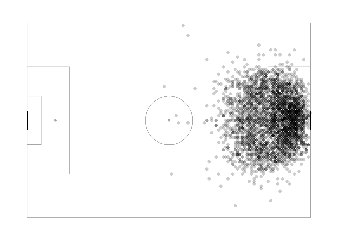
Figure 1: Darker regions imply more shots
Central locations a few yards from goal seem like prime real estate for taking shots. Which is pretty intuitive. Being closer to goal when shooting makes it a lot easier to score. Lesser time for the goalkeeper to react, lesser defenders to block your attempt at goal. In fact, it’s easily the most important information that the model will need. Statsbomb provides me with the x and y coordinate of the pitch location from which the shot was taken. They also provide me with the coordinates of the goalkeeper at the time the shot was taken. So I thought I’ll create a few variables to represent this information.
shots_valid = shots_valid %>% mutate(opposite = 120 - location.x,
                                                adjacent = 40 - location.y,
                                                hypotenuse = sqrt(opposite^2 + adjacent^2),
                                                angle.to.goal = ifelse(location.y > 40, 180 - asin(opposite/hypotenuse)*180/3.14, asin(opposite/hypotenuse)*180/3.14),
                                                distance.to.goal = hypotenuse) %>%
                                                  select(-c(opposite, adjacent, hypotenuse))
I calculated the angle of a shot to goal as the angle between the goal line and the line joining the center of the goal to position of the shot2. The distance to goal was merely the length of the latter line. (The statsbomb pitch is 120 units long and 80 units wide (their document states these can be thought of as yards - with link). The coordinate of the center of the goal is (120, 40)).
For example, the angle to goal from a shot taken from (100,55) looks like this -
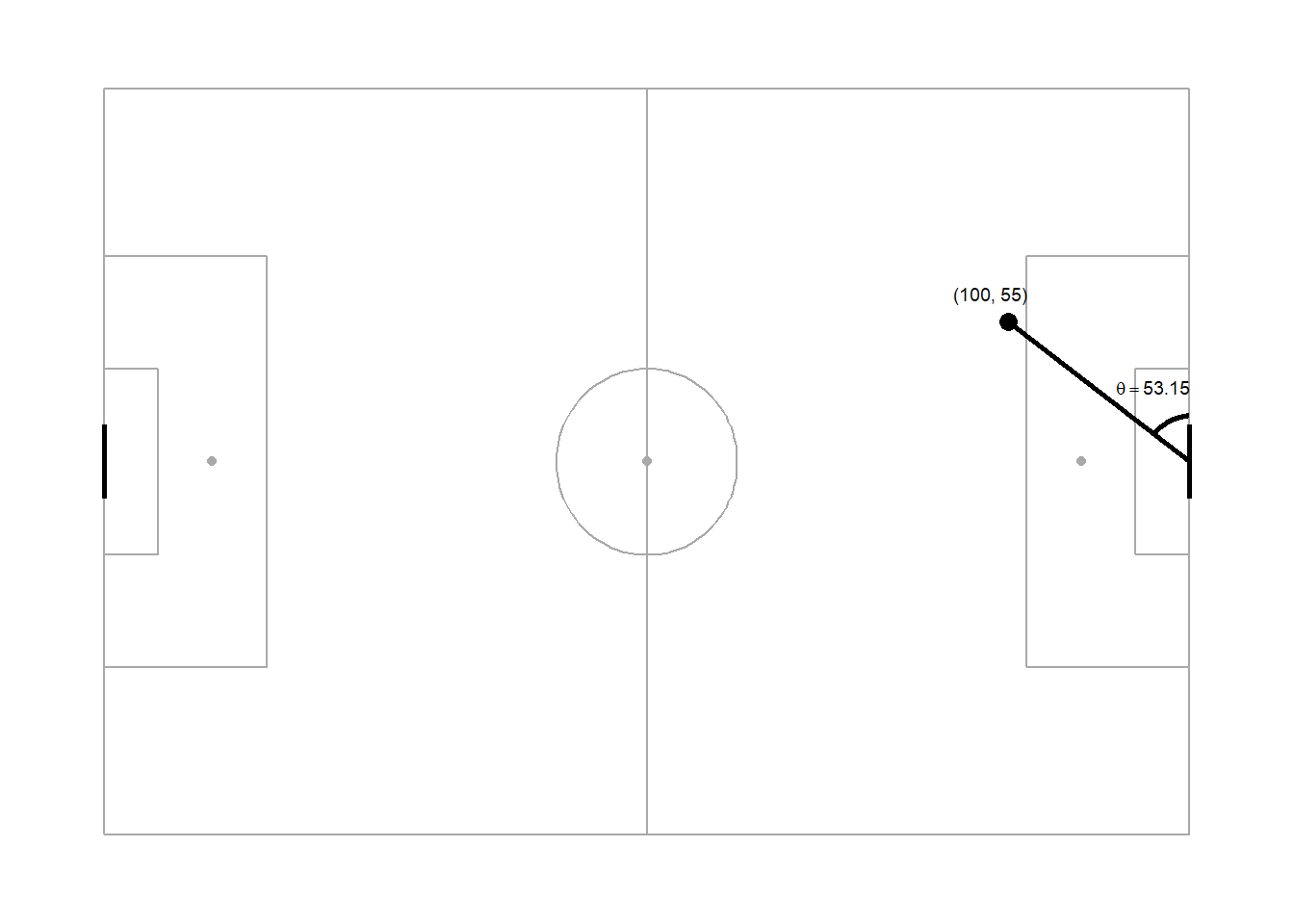
Figure 2: A shot taken from (100, 55) is taken at an angle of 53.15 degrees to goal
I did something similar for distance and angle to goalkeeper, adding a few cavaets for the few situations in which the shooter was ahead of the goalkeeper.
#adding distance from goalkeeper and angle to gk
shots_valid = shots_valid %>% mutate(opposite = location.x.GK - location.x,
                                                adjacent = location.y.GK - location.y,
                                                hypotenuse = sqrt(opposite^2 + adjacent^2),
                                                angle.to.gk = ifelse(location.y > location.y.GK, 180 - asin(opposite/hypotenuse)*180/3.14, asin(opposite/hypotenuse)*180/3.14),
                                                angle.to.gk = ifelse(location.x > location.x.GK & location.y < location.y.GK, 270 - asin(opposite/hypotenuse)*180/3.14, angle.to.gk),
                                                distance.to.gk = hypotenuse,
                                                gk.to.goalline = sqrt((120 - location.x.GK)^2 + (40 - location.y.GK)^2)) %>%
                                                  select(-c(opposite, adjacent, hypotenuse))
At this point, I have all the information I need to build a basic xG model. I chose random forest as my model of choice because:
- They’re quite stable
- They don’t make any assumptions about the data
- They’re easy to build
- I wouldn’t rule out being biased towards them after reading a Statsbomb whitepaper which detailed the construction of their own xG model using Random Forests
Statbomb’s data is quite clean and did not require much cleaning, but they have a few random shots missing information on goalkeeper position. I plotted the shots with missing data and looked for patterns through various ‘color’ variables, but no pattern leapt out. Since these were only 60 shots, I removed them from the data.
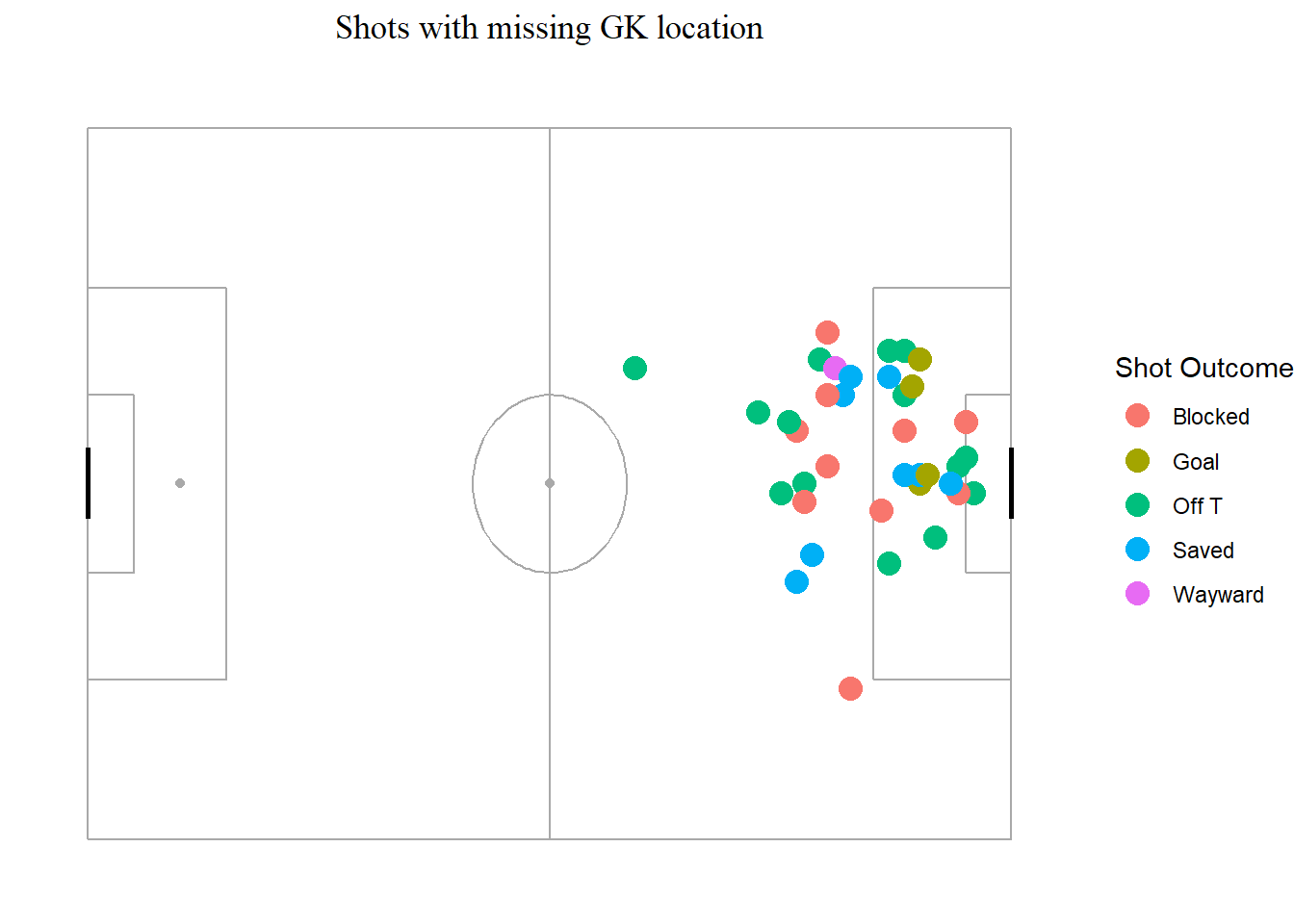
Figure 3: Missing shots had no pattern I could discern
Building the model
#choosing independent variables
ind.vars = c('id', 'is.goal','distance.to.gk', 'distance.to.goal', 'angle.to.gk', 'angle.to.goal', 'gk.to.goalline', 'play_pattern.name','shot.body_part.name', 'shot.type.name', 'shot.technique.name')

shots.varsdata = subset(shots_valid, select = ind.vars) %>% drop_na()

#splitting into test train
idx = createDataPartition(shots.varsdata$is.goal, p = 0.8, list = F)
train = shots.varsdata[idx,]
test = shots.varsdata[-idx,]
vars = ncol(model.matrix(is.goal ~ ., train[,!colnames(train) %in% c("id")])) - 2
grid = expand.grid(mtry = 4:vars)
control = trainControl(classProbs = TRUE, method = "cv", number = 5,
allowParallel = T,summaryFunction = prSummary, savePredictions = T)
rf.1 = caret::train(is.goal ~ .,
data = train[,!colnames(train) %in% c("id")],
method = "rf",
metric = "F",
trControl = control,
tuneGrid = grid,
preProcess = c("center", "scale"))
xG_test.rf.v1 = predict(rf.1, test, type = "prob")My first xG model was based completely on location information3. Additional context was provided by body part the shot was taken with, state of play (open play, corner..) and shot technique (header, volley..). It had a AUC-PR of 0.25, AUC-ROC was 0.7 and an F-score of 0.18. I’m sure I can increase this by 5-7 points just by providing my model with more data.
This model primarily used information about location of the shooter and the goalkeeper to estimate the chance of a shot becoming a goal. There are other indicators that can help build a better representation of a goal scoring situation. I built a couple of them to help this model.
Building other variables to capture the context of a shot
The first is looking at throughballs. Succesful throughballs usually find their target with space to run into, leaving the defenders scrambling. Other models I have read about have looked at whether a throughball was played in a 5 or 10 second window before a shot. I didn’t create a similar window as I was not confident of estimating it accurately with the data I’m using. So I created two variables, one to look at whether a throughball was played in an attack that lead to a shot, and another measuring the seconds between the throughball and the shot. As I add more data, the model should be able to figure out how long before a shot a throughball should be played for it to be meaningful.
The second was successful dribbles. Players who have dribbled past a defender usually have more time to pick out a neat pass or shoot precisely. I added a couple of similar variables to capture this information.
Both these ideas, along with several others, were explored in this xG model explanataion article, written way back in 2015 by Michael Caley.
#Flagging all possessions with a through ball and dribbles
all_events = all_events %>% group_by(match_id, possession) %>%
  mutate(tb.flag = any(pass.through_ball == T),
         shot.flag = any(type.name == 'Shot'),
         dribble.flag = any(dribble.outcome.name == 'Complete'),
         tb.time = ifelse(shot.flag == T & pass.through_ball == T, TimeInPoss, NA),
         shot.time = ifelse(type.name == 'Shot', TimeInPoss, NA),
         dribble.time = ifelse(shot.flag == T & dribble.outcome.name == 'Complete', TimeInPoss, NA)) %>%
  fill(tb.time, shot.time, dribble.time) %>%
  mutate(dribble.to.shot.time = shot.time - dribble.time,
         tb.to.shot.time = shot.time - tb.time)
Do these new variables work? Do they mean anything? It’s easy to perform a non-robust eye test -
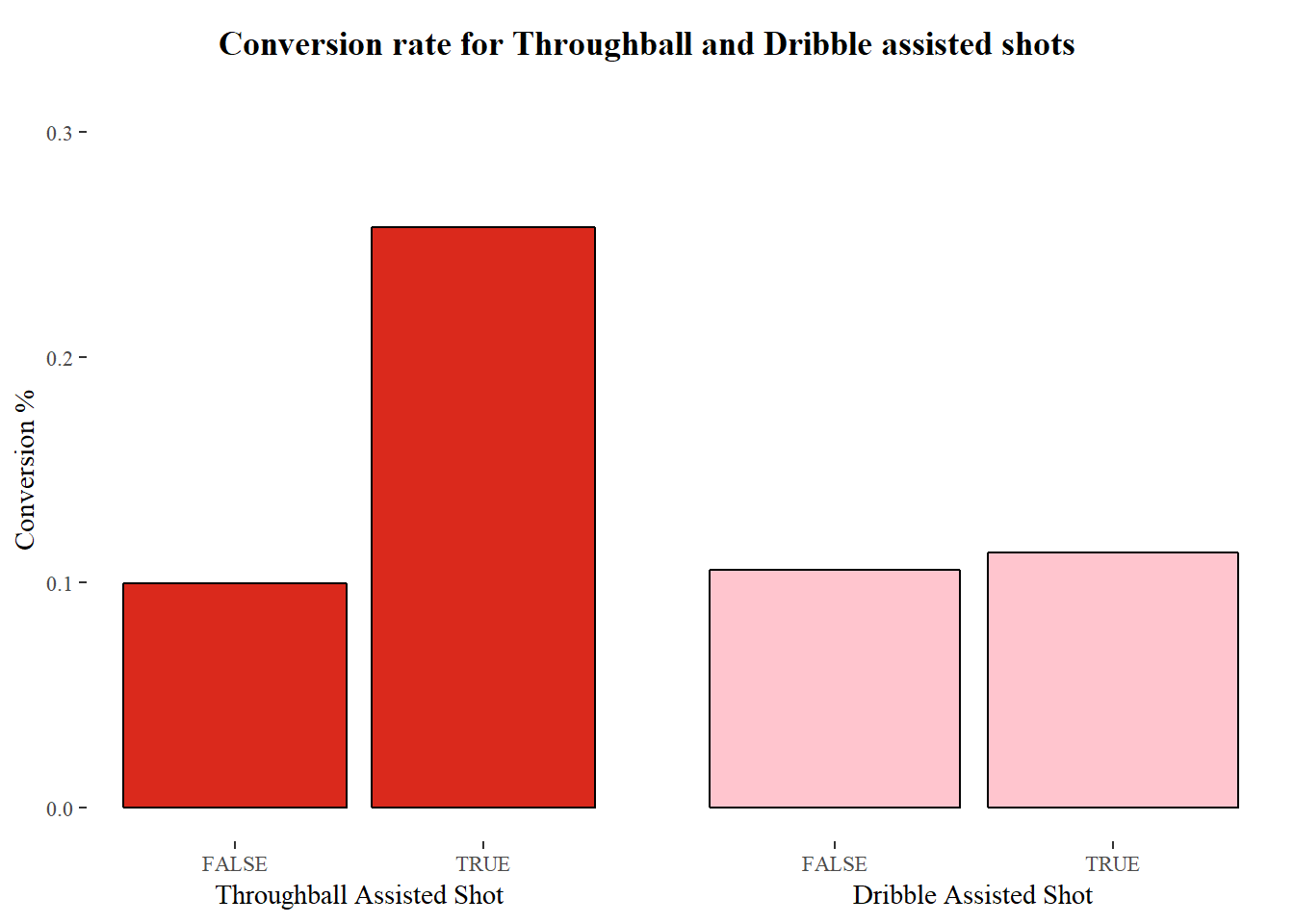
Throughball assisted shots have a significantly high conversion rate. Dribbles, not so much, but I’m positive these two variables should improve the model.
One problem I encountered here was NA values in tb.to.shot.time, which measured the seconds between a throughball being played and a shot taken in the same possession sequence. Obviously, this value was NA whenever there was no throughball in a sequence with a shot. The NA value was completely valid in this context and provided information about the absence of a throughball. But since my model did not accept NA values in the data, I replaced them with an arbitrary high value (5000) to indicate the absence of a throughball. The model shouldn’t confuse this to be a valid value, as valid values for tb.to.shot.time maxes out at 44.96 seconds.
Did including the new variables improve the performance of the model? Slightly. AUC-ROC was 0.72, AUC-PR was 0.26 and the F-score was 0.20. I expected a more stark improvement, but the handicap could be data more than anything else. There is some support for this, given that out of the 3300 shots taken, only 128 of them had a throughball in their buildup.
Exploring the results
To compare the model’s performance with one another, I’ll use ROC curves. In short, the model whose line covers the most area in the ROC plot has the best performance. A perfect model will cover all the area (touch the top left corner, Area Under Curve = 1). I’ll also add Statbomb’s model to the mix.
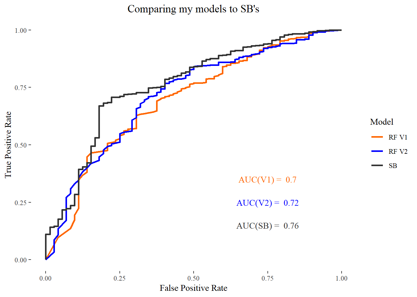
Providing the model with more context about the shot (V2), helped it outperform one without such information (V1). I included Statsbomb’s own model here for a comparison, and although it may not look it here, it completely smokes mine. Creating other context capturing variables to inch closer to their performance will a interesting future project.
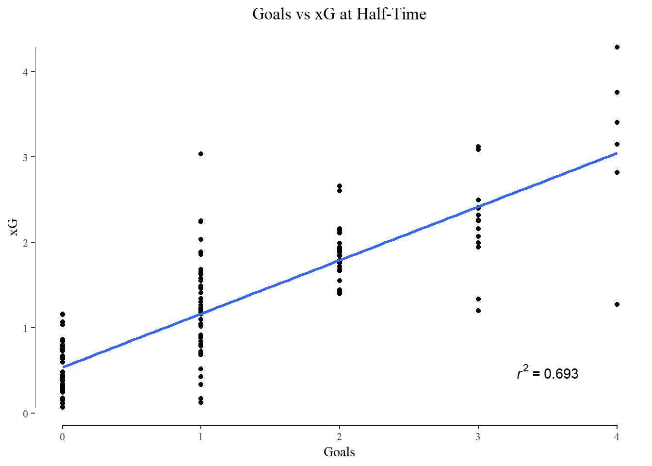
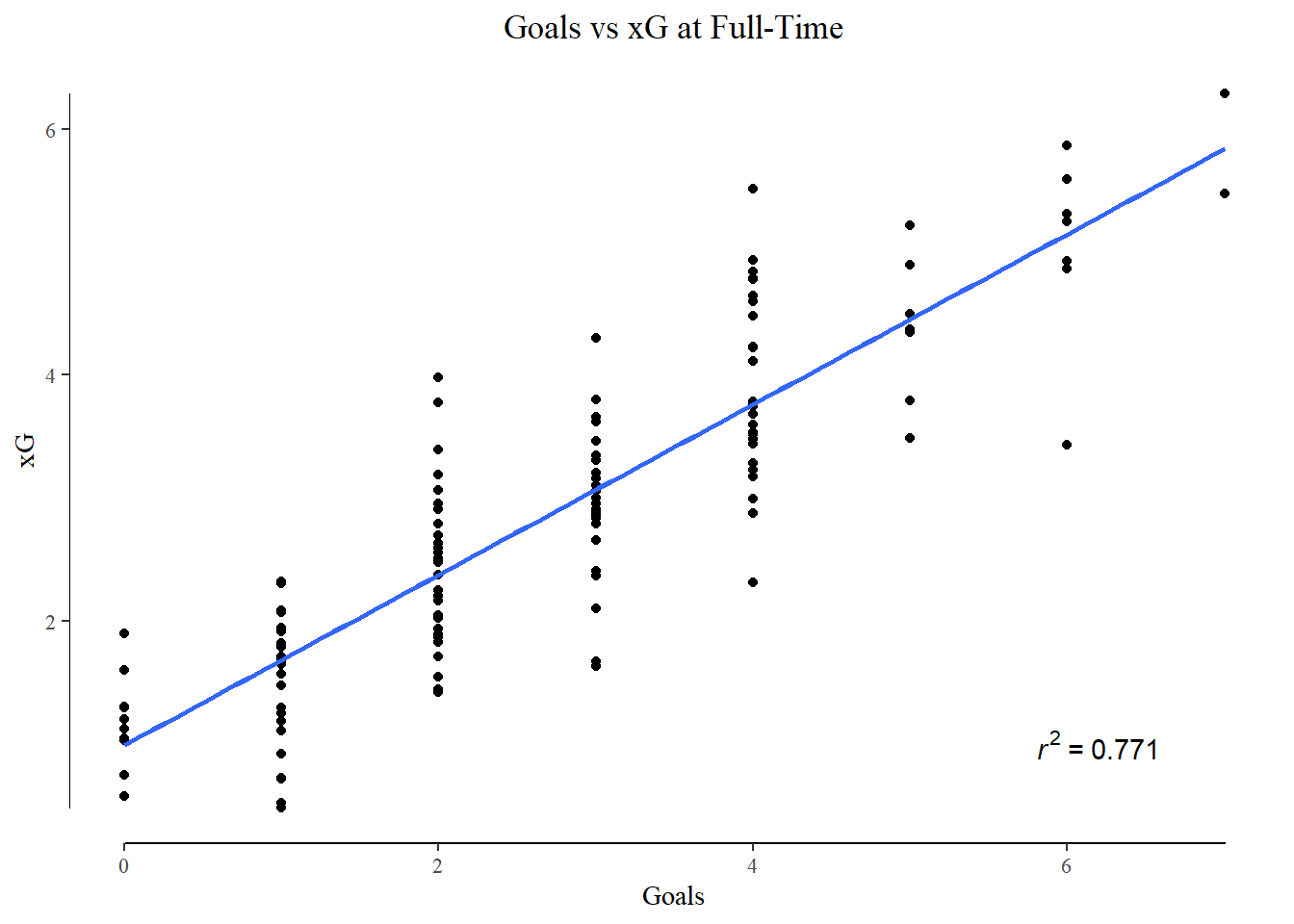
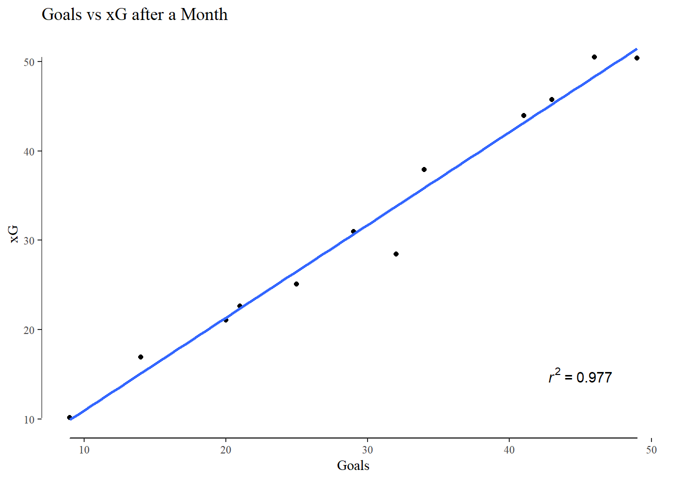
Despite its simplicity, my model held up quite well to matching goals scored over the long term. Which, like this article says, is the main goal of xG -
“Notably what xG was not developed to do is accurately describe a single shot or a single game. Rather, it was designed to take lots of information, thousands and thousands of shots, synthesize it, and use that information to represent how many goals a team might reasonably be expected to score or concede given the types of shots they’ve taken and given up.”
I measured xG’s ability to predict actual goals scored in one half, match, week, and month of football. On cue, their predictive ability increased as the time frame lengthened.

Looking at the shot map I created early in the article, and coloring the shots with their xG -
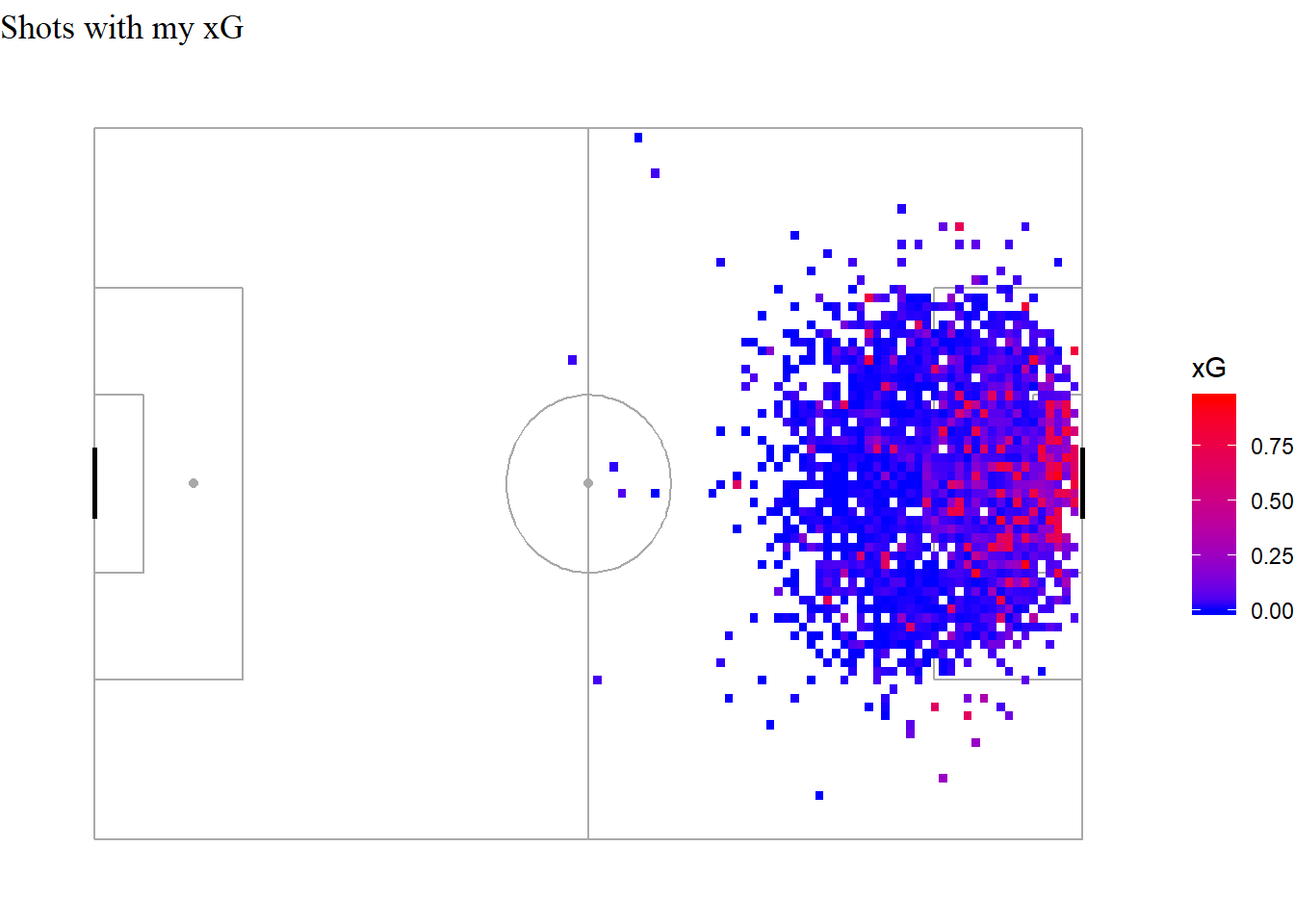
An easy eye-test plot to judge the performance of my model. Although it performs decently well on aggregated shot totals over a few months, I think it’s weakness in single shot xG really stands out here. There are quite a few shots from extreme angles and locations that it has assigned a high xG value to. I presume this is due to a lack of shots from these locations, with the existing ones presenting a picture of a high conversion area.

Building the same map with Statsbomb’s xG shows how well calibrated their model is. There’s a gradual decrease in xG as we move away from goal. In comparison, there are quite a few zones in the box where my model is either very optimistic about a shot, or quite unbearably pessimistic.
Improving my model’s estimation of single shot xG will be my next target. I’ll iterate over this model, add some variables to improve it (like game state). I’m thinking my other projects with this data will be:
Quantify the value of the location each pass is played from (build an xPass model)
Test the ‘hot hand’ hypothesis
Thanks for reading! All code used in this article can be found here
Footnotes
This wasn’t the original point of expected goals. It was a replacement for shot totals and shot ratios in predicting the long term performance of a team. xG is pretty good at predicting how a team will do in the future, given long term data. Single match xG totals are more unstable and are rarely used as a lone stat to judge games.↩
The angle I am finding is \(\theta\), and \(sin\theta = \frac{opposite}{hypotenuse}\). Opposite is given by the line from goalline to the location of shot (parallel to the touchline). Hypotenuse I get from the Pythagoras theorem (\(hypotenuse^2 = opposite^2 + adjacent^2\))↩
I used 5-fold cross validation, tuned for
mtry(optimum number of trees at each split) and used F-scores to pick the best model. I preferred F-scores and AUC-PR values to evaluate my model over the more popular AUC-ROC values due to the imbalanced nature of soccer shots datasets. Goals are a rare event, and it is easier for the model to predict a negative (goal not scored) rather than a positive. In such cases, AUC-ROC presents an optimistic picture of a model’s performance as it accounts for true negatives, which are easier to get right than true positives. Since both precision and recall do not care for TN, they do not have this bias.↩